This blog post is part of a series describing my ongoing analysis of the Kaggle Horses For Courses data set using Azure Data Lake Analytics with U-SQL and Azure Notebooks with F#. This is part 4.
- Horses For Courses data set analysis with Azure Data Lake and U-SQL
- Horses For Courses barrier analysis with Azure Notebooks
- Kaggle Horses for Courses age analysis with Azure Notebooks
- Kaggle Horses for Courses analysis of last five starts with Azure Notebooks (this blog post)
Data set and recap
A quick recap of Kaggle and the data set we're analyzing: Horses For Courses. Kaggle is a data science and machine learning community that hosts a number of data sets and machine learning competitions, some of which with prize money. 'Horses For Courses' is a (relatively small) data set of anonymized horse racing data.
In the first post I discussed how you could use Azure Data Lake Analytics and U-SQL to analyze and process the data. I used this mainly to generate new data files that can then be used for further analysis. In the second and third post I studied the effects of barrier and age on a horse's chances of winning a race.
In this post I'm going to study the relation between the last five starts that is known before a horse starts a race and its chances of winning the race. For every horse in a race we know the results of its previous five races from the runners.csv file in the Kaggle dataset. At first sight, this seems a promising heuristic for determining how a horse will perform in the current race so let's see if that's actually the case.
The analysis itself will again be performed using Azure Notebooks with an F# kernel. Here's the link to my notebook library.
What data are we working with?
A typical last five starts might look like this: 3x0f2. So what does this mean? A short explanation:
1to9: horse finished in position 1 to 90: horse finished outside the top 9f: horse failed to finishx: horse was scratched from the race
So in 3x0f2 a particular horse finished third, was scratched, finished outside the top 9, failed to finish and finished second in its previous five races.
You may already spot a problem here. When we get a 1 to 9, we know what happened in a previous race. When we get a 0, we have some information but we don't know exactly what happened. For an f or an x we know nothing. In both cases, if the horse had run, it might have finished at any position.
To be able to compare the last five starts of two horses, we have to fix this. Especially, if we want to use this data as input to a machine learning algorithm, we should fix this1.
When we do some more digging in the dataset, it appears that we do not have a complete last five starts for every horse. For some horses, we only have the last four starts or the last two. And for some horses we have nothing at all. Let's take a look at the distribution of the length of last five starts in our dataset:
(5: 72837) (4: 3379) (3: 3461) (2: 3553) (0: 5054)
I've written it a down a bit terse but you can see that for 72837 (or 83% of) horses we know the last five starts. But still, it's hard to compare 32xf6 with 4f so we should fix the missing data as well.
Fixing the data
The accompanying Azure Notebook describes all fixes in detail, so I'll give a summary here:
xandf: In both cases, a horse could have finished the race but didn't2. What we do here is replace eachxandfwith the average finishing position of a horse over all races as a best guess (we can simply take the average over all races of the number of horses in a race).0: The horse finished outside the top 9 so we replace each0with the average finishing position for horses outside the top 9 (and here we take the average over all races with more than 9 horses).- missing data: This is essentially the same as not starting or failing to finish so we take the average finishing position again.
One small example of what's happening: suppose we have 4xf0. With our current algorithm, this will be represented as (4.00, 6.49, 6.49, 11.66, 6.49) as follows:
4 | → | 4.00 | A 4 will remain a 4. |
x | → | 6.49 | An x will be replaced by 6.49, the average finishing position over all races. |
f | → | 6.49 | An f will be replaced by 6.49, the average finishing position over all races. |
0 | → | 11.66 | A 0 will be replaced by 11.66, the average finishing position for horses that finish outside the top 9. |
| missing data | → | 6.49 | Missing data will be replaced by 6.49, the average finishing position over all races. |
Comparing last five starts
Now that we can be sure that every last five starts has the same length, how do we compare them? The easiest way in my opinion is to take the average. So with our previous example we get:
4xf0 → (4.0, 6.5, 6.5, 11.7, 6.5) → 7.04
And we can do this for every horse. So now we have one number for every horse in a race that describes the last five starts, how convenient :) 3
Preparing the data file
With fixing and averaging in place, we will use switch back to U-SQL to prepare our dataset. Remember from the first post that we want pairs for all horses in a race so that we can reduce our ranking problem (in what order do all horses finish) to a binary classification problem (does horse a finish before or after horse b).
I'll digress a bit into Azure Data Lake and U-SQL so if you just want to know how last five starts relates to finishing position you can skip this part. I'm assuming you already know how to create tables with U-SQL so I'll skip to the part where I create the data file we will use for analysis.
First of all, we need the average finishing position over all races so we can fix x, f and missing data:
@avgNrHorses =
    SELECT (((double) COUNT(r.HorseId)) + 1d) / 2d AS AvgNrHorses
    FROM master.dbo.Runners AS r
    GROUP BY r.MarketId;
@avgPosition =
    SELECT AVG(AvgNrHorses) AS AvgPosition
    FROM @avgNrHorses;
We get the average number of horses in each race and than calculate the average over that. Second, we need the average finishing position of horses outside the top 9:
@avgNrHorsesAbove9 =
    SELECT
        (((double) COUNT(r.HorseId)) - 10d) / 2d AS AvgNrHorses,
        COUNT(r.HorseId) AS NrHorses
    FROM master.dbo.Runners AS r
    GROUP BY r.MarketId;
@avgPositionAbove9 =
    SELECT AVG(AvgNrHorses) + 10d AS AvgPosition
    FROM @avgNrHorsesAbove9
    WHERE NrHorses > 9;
A little more complex but essentially the same as the previous query but with just the races that have more than 9 horses.
The final part is where we generate the data we need and output it to a CSV file:
@last5Starts =
  SELECT
    HorsesForCourses.Udfs.AverageLastFiveStarts(
      r0.LastFiveStarts, avg.AvgPosition, avg9.AvgPosition) AS LastFiveStarts0,
    HorsesForCourses.Udfs.AverageLastFiveStarts(
      r1.LastFiveStarts, avg.AvgPosition, avg9.AvgPosition) AS LastFiveStarts1,
    p.Won
  FROM master.dbo.Pairings AS p
  JOIN master.dbo.Runners AS r0
    ON p.HorseId0 == r0.HorseId AND p.MarketId == r0.MarketId
  JOIN master.dbo.Runners AS r1
    ON p.HorseId1 == r1.HorseId AND p.MarketId == r1.MarketId
  CROSS JOIN @avgPosition AS avg
  CROSS JOIN @avgPositionAbove9 AS avg9;

OUTPUT @last5Starts
TO "wasb://output@rwwildenml.blob.core.windows.net/last5starts.csv"
USING Outputters.Csv();
There are two interesting parts in this query: the AverageLastFiveStarts function call and the CROSS JOIN. First the CROSS JOIN: both @avgPosition and @avgPositionAbove9 are tables with just one row. A cross join returns the cartesian product of the rowsets in a join so when we join with a rowset that has just one row, this row's data is simply appended to each row in the first rowset in the join.
The AverageLastFiveStarts user-defined function takes a last five starts string, fixes it in the way we described earlier and returns the average value:
namespace HorsesForCourses
{
  public class Udfs
  {
    public static double AverageLastFiveStarts(string lastFiveStarts,
                                               double? avgPosition,
                                               double? avgPositionAbove9)
    {
      // Make sure the string has a length of 5.
      var paddedLastFiveStarts = lastFiveStarts.PadLeft(5, 'x');
      var vector = paddedLastFiveStarts
        .Select(c =>
        {
          switch (c)
          {
            case 'x':
            case 'f':
              return avgPosition.Value;
            case '0':
              return avgPositionAbove9.Value;
            case '1': case '2': case '3': case '4': case '5':
            case '6': case '7': case '8': case '9':
              return ((double) c) - 48;
            default:
              throw new ArgumentOutOfRangeException(
                "lastFiveStarts", lastFiveStarts, "Invalid character in last five starts");
          }
        });
      return vector.Average();
    }
  }
}
The code is also up on Github so you can check the details there.
Analysis
We now have a data file that has, on each row, the last five starts average for two horses and which of the two won in a particular race. Some example rows:
3.90, 6.49, True
4.30, 6.49, False
6.70, 3.50, False
6.70, 5.40, False
7.63, 4.40, False
6.69, 5.49, True
On the first row, a horse with an average last five starts of 3.90 beat a horse with an average last five starts of 6.5. On the second row, 4.3 got beaten by 6.5, on the third row, 6.7 got beaten by 3.5, etc.
So how do we get a feeling for the relation between last five starts and the chances of beating another horse. I decided to do the following:
- Get the largest absolute difference between last five starts for two horses over the entire data set.
- Get all differences between last five starts pairs.
- Distribute all differences into a specified number of buckets.
- Get the numbers of wins and losses in each bucket and calculate a win/loss ratio per bucket.
In the example rows above, the largest difference is in row 5: 3.23. Since differences can be both positive and negative, we have a range of length 3.23 + 3.23 = 6.46 to divide into buckets. Suppose we decide on two buckets: [-3.23, 0) and [0, 3.23]. Now get each difference into the right bucket:
                    diff        bucket
3.90, 6.49, True,  -2.59  --> bucket 1
4.30, 6.49, False, -2.19  --> bucket 1
6.70, 3.50, False,  3.19  --> bucket 2
6.70, 5.40, False,  1.29  --> bucket 2
7.63, 4.40, False,  3.23  --> bucket 2
6.69, 5.49, True,   1.20  --> bucket 2
So we have 2 horses in bucket 1 and 4 horses in bucket 2. The win/loss ratio in bucket 1 is 1 / 1 = 1, the win loss ration in bucket 2 is 1 / 4 = 0.25. So if the difference in last five starts is between -3.23 and 0, the win/loss ratio is 1.0. If the difference is between 0 and 3.23, the win/loss ratio is 0.25.
This is of course a contrived example. In reality we have almost 600000 rows so we will get some more reliable data. I experimented a little with bucket size and 41 turned out to be a good number. This resulted in the following plot. I skipped the outer three buckets on both sides because there aren't enough data points in there.
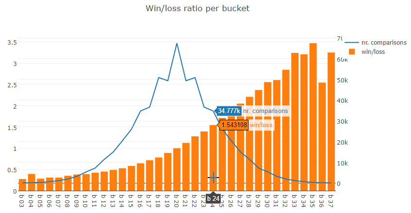
The bars represent the buckets, the line represents the number of data points in each bucket. I highlighted bucket 24 as an example. This bucket represents the differences between average last five starts of two horses between 1.59 and 2.05. This bucket has 34777 rows and the win/loss ratio is 1.54.
This means that if the difference between average last five starts of two horses is between 1.59 and 2.05, the horse with the higher average is 1.54 times more likely to beat the other horse! This is pretty significant. If we take two random horses in a race, look at what they did in their previous five races and they happen to fall into this bucket, we can predict that one horse is 1.54 times more likely to win.
We need to put these numbers a little bit into perspective, because it matters how many records of the total population fall into bucket 24. This is about 5.83%. However, the data set is symmetric in the sense that it includes two rows for each horse pair (so if we have a,b,True we also have b,a,False). So bucket 16 is the inverse of bucket 24 with the same number of records: 34777. This means we can actually tell for 11.66% of the total population that one horse is 1.54 times more likely to win than another horse.
Conclusion
So far, we have analyzed three features for their effect on horse race outcomes: barrier, age and last five starts. Barrier and age had a clear effect and now we found that average last five starts also has an effect. Each one of these separately cannot be used to predict horse races but maybe combined they present a better picture.
Age and barrier are independent of each other. The barrier you start from is the result of a random draw and it has no effect on the age of a horse. Vice versa, the age of a horse has no effect on the barrier draw. We already established that both age and barrier have an effect on race outcomes so you might be inclined to think that both also have an effect on the last five starts. This is not true for barrier but it may be true for age. We determined in the previous post that younger horses outperform older horses. It makes sense then that the last five starts of younger horses is better than that of older horses.
Ideally we would like to present a machine learning algorithm a set of independent variables. Using both age and last five starts may not be a good idea.
In the next post we'll get our hands dirty with Azure Machine Learning to see if we can get 'better than random results' when we present the features we analyzed to a machine learning algorithm. Stay tuned!
Footnotes
- Actually there is no machine learning 'law' that requires us to fix the data. We could just leave the
x,fand0as they are and have the algorithm figure out what they mean. However, think about what this would mean. Suppose we have two horses:067xfand9822xand the first won. The input for our machine learning algorithm would be:0,6,7,x,f,9,8,2,2,x,True. That's 10 feature dimensions, just to describe the last five starts! High-dimensional sample spaces are a problem for most machine learning algorithms and this is usually referred to as the curse of dimensionality, very nicely visualized in these two two Georgia Tech videos. So the less dimensions, the better. - You could argue that being scratched from a race (
x) and failing to finish (f) are two different things. Especially anfcould give us more information about future races. Suppose we see the following last five starts:638ff. The horse failed to finished in its last two races. This doesn't give much confidence about the current race. On the other hand,f8f63tells a different story but has the same results, just in a different order. Maybe in a future blog post I'll dig deeper into better methods for handlingxandf. - I have given some thought to other ways of comparing last five starts but averaging is at least the simplest and maybe the best solution. You could argue that trends should be taken into account so that
97531is better that13579. The first shows a clear positive, the second a clear negative trend. However, deriving a trend from a series of five events seems a bit ambitious so I decided against it.